How to highlight alternate rows in Excel 2013

Highlighting alternate rows in Excel 2013 worksheet makes the data visually much more appealing. Instead of doing this manually, we can use Conditional Formatting feature to automatically shade every other row in Excel.

Conditional Formatting gives us flexibility to change the shade colour in case it is required. The biggest advantage of using Conditional Formatting is that the shading is dynamic i.e. it automatically updates if we insert or delete the rows.

Also read: How to Trace Precedents and Dependents in Excel 2013

Below steps will help you highlight alternate rows:

1. Select the data range where we want to highlight alternate rows.
   

2. Go to "HOME" tab >>> Conditional Formatting >>> Click "New Rule..."
   

3. This will open conditional formatting dialog box. Click "Use a formula to determine which cells to format"

4. Enter the formula =MOD(ROW(), 2)
   

5. Click on "Format" button and choose the shade or format for alternate rows
   

6. Click OK >> OK and you will see that alternate rows in selected data range are shaded as per desired format (here with GREEN fill)
   

More interesting articles on this website:

• How to use AGGREGATE function in Excel 2013
• Two Way lookup in Excel 2013 using INDEX and MATCH
• How to create Histogram in Excel 2013
• How to create Waterfall Chart in Excel 2013

How to find and highlight cells with formula in Excel 2013

Excel 2013 has introduced some awesome new functions that can help professionals save time.

Some of the amazing new functions include: DAYS, IFNA, ISFORMULA, XOR, ISOWEEKNUM and many more.

Also read: Top 7 new features in Excel 2013 that every professionals must know

The new ISFORMULA function detects if the cells contains formula. We can use CONDITIONAL FORMATTING along with ISFORMULA function to identify and highlight cells containing formula.

Syntax: ISFORMULA (reference)

• Reference can be a cell reference, a formula, or even a name that refers to a cell.

Suppose we have data-set as shown below, with expense occurred in each month and column H have formula for total expenses.

Follow the below steps to identify and highlight cells with formula:

1. Select cell range A4:H4 and keep A4 as active cell
   
2. Go to "HOME" tab >>> Conditional Formatting >>> Click "New Rule..."
   
3. This will open conditional formatting dialog box. Click "Use a formula to determine which cells to format"
4. Enter ISFORMULA function giving reference to active cell (here A4 cell) =ISFORMULA(A4)

   

   
   
5. Click on "Format" button and choose the format for the cells with formula
   
6. Click OK >> OK and you will see that all cells with formula are coloured with desired format (here with GREEN fill)
   

More interesting articles on this website:

• How to create Two-Variable Data Table in Excel 2013
• Two Way lookup in Excel 2013 using INDEX and MATCH
• How to freeze panes in Excel 2013
• How to create Waterfall Chart in Excel 2013

Top 7 new features in Excel 2013 that every Professional must know

Flash Fill feature
"Flash Fill" is the magical feature introduced in Excel 2013

Flash Fill detects a pattern in your initial data entry which enables it to figure out remaining data you want to enter.

For example, combining first names and last names from different columns is detected by Flash Fill and applied across multiple rows based on pattern detection.

Also read: How to split first and last names in Excel 2013 using Flash Fill 

Chart Recommendations

Now this is pro-active feature launched by Excel 2013!! Based on the selected data, Excel recommends appropriate chart which makes it more intuitive.

Follow below steps to use this feature:

1. Select the data >>> Go to "INSERT" tab >>> select "Recommended Charts"
   
2. This will open a dialog with range of charts. The interesting part is we can click on each chart and see the preview of that chart.
   
3. Choose the desired chart and hit OK. Your chart is ready!!

Quick analysis Tool

This is again an excellent tool introduced in Excel 2013 to preview the data in insightful ways.

In order to use this tool, select the data you want to analyze and instantly the Quick Analysis icon appears at the bottom-right corner. This tool has lot of design and formatting options which is worth exploring. Additionally, it provides preview before actually applying any option.

Extensive Cloud support with SkyDrive

Excel 2013 allows users to share their Excel workbooks on SkyDrive. This enables quick and easy access to your Excel files on any device running Excel 2013 (which can include your windows tablet, smartphone, desktop or laptop).

Also, with Office 365 subscription one can review and edit workbooks online using almost any web browser.

Sharing on Social Networks

This is an innovative feature introduced keeping in mind the growing use of Social Networks. 

To share Excel files on Social Networks follow below steps:

1. Go to "FILE" >>> Share >>> Post to Social Networks
2. Select any social network that is linked with your Office 2013 account
3. Select privacy options of read-only or edit for the shared worksheet
4. Include any message in the message box and press "POST" button

Pivot Tables Recommendation

Pivot Tables helps immensely for data analysis and managerial decisions, but most of us usually face difficultly in effectively using it. Excel 2013 has almost solved this problem by introducing "Recommended Pivot Tables" feature.

Again, it’s extremely easy to use it:

Click inside data range >>> Go to "INSERT" tab >>> Recommended PivotTables

This will open a dialog box showing the list of recommended pivot tables along with explanations.

Select the table which suits your output and press OK. It's done!!

Introduction of great new functions

What's more!! Excel 2013 has introduced some awesome functions that can help professionals save time.

Some of the amazing new functions include:

• DAYS – returns the number of days between two dates
• IFNA – returns specific value if the formula gives #N/A error
• ISFORMULA – detects the cells containing formula
• XOR – detects expressions and returns FALSE only when all expressions are FALSE
• ISOWEEKNUM – returns ISO week for a date

Please comment, SHARE or LIKE if you enjoyed this article!! Visit Facebook page: FundooExcel

More interesting articles on this website:

• Text Alignment keyboard shortcuts for Excel 2013
• How to freeze panes in Excel 2013
• How to generate RANDOM number in Excel 2013
• How to create two-variable Data Table in Excel 2013

How to transpose rows and columns in Excel 2013

Download Excel File

TRANSPOSE literally means changing the orientation of a cell range or an array.  Thus, TRANSPOSE enables to swap data from rows into columns and vice-versa.

We can transpose the data in Excel 2013 in two ways:
1. Static Transpose – using "Paste Special"
2. Dynamic Transpose – using TRANSPOSE function

Static Transpose using "Paste Special" function

This method is very useful when we have to quickly transpose data without changing anything in the future. The output data is STATIC i.e. it does not have any linking or formula attached to it.

Following steps will be helpful for static transpose using paste special option:

1. Select the cell range that you want to transpose and copy the same (Ctrl+C)

2. Select the cell where you want the output to start

3. Go to "Home" tab >>> "Paste" button >>> Paste Special >>>Transpose

OR  Right click >>> Paste Special >>> Transpose
Shortcut: Ctrl+Alt+V >>E  OR Alt+ESE

4. Press OK and its done. The transposed data will get pasted starting from the selected cell.

Dynamic Transpose using TRANSPOSE function

TRANSPOSE function gives the output with linking. Hence, if the original data altered, the transposed data will reflect the change automatically.

TRANSPOSE function is an "Array" function i.e. it takes cell range as input (quite logical..!!) and needs combination of "Ctrl + Shift + Enter" keys to insert. Array functions are enclosed by curly braces {}.

One critical difference between Paste Special and TRANSPOSE function:

For using TRANSPOSE function the output range should be selected first and it should be an appropriate array/cell range i.e. if the input range is 2x3 cell range, the output range selected should be 3x2 cell range.

1. Select the output cell range where the transposed data is required. You can watch the selection matrix in the "Name Box".

2. Keep the cell range selected and type below formula:

       =TRANSPOSE (input cell range)

       "input cell range" is the input data range which we want to transpose

3. Press "Ctrl + Shift + Enter" after entering the formula. This will automatically enclose formula with curly braces {}.

Important Note: Once the TRANSPOSE function is applied, you cannot edit or delete any of the individual cells in the output range.

How to insert current date and time in a cell in Excel 2013

Download Excel File

When we work in Excel, we sometimes require to enter current date or time. The purpose may be to maintain log of activities or tracking some changes.

There are mainly two methods to insert current date & time in a cell in Excel 2013:     

1. Dynamic – A date or time that updates when the worksheet is recalculated
2. Static – A value in worksheet that doesn't change

Inserting "DYNAMIC" date and time

TODAY and NOW functions are generally used to insert dynamic current date and time respectively.

Syntax for the TODAY function is:

=TODAY()

NOW function is used to insert "current time" which is dynamic

Syntax for NOW function is very similar to TODAY:

=NOW()

Important Note: As you might have noticed, these functions have no arguments i.e. () does not contain anything. As a result, the data updates each time the worksheet is recalculated.

Inserting "STATIC" date and time

Select the cell into which you want to insert current date or time

To insert current date >>> Press CTRL + semi-colon (;)

To insert current time >>> Press CTRL + SHIFT + semi-colon (;)

To insert both date and time >>> Press CTRL + semi-colon (;), then press SPACE and then CTRL + SHIFT + semi-colon (;)

Important Note: In both the above cases, Excel will give date format as per the default settings. You can change the format from cell format menu [Shortcut: "Ctrl+1"] in "Number" tab >> Date

How to use RANK function in Excel 2013

The RANK function returns the rank of a number, i.e. its position within a list of numbers in Excel 2013. We will also look into RANK.EQ and RANK.AVG functions which are introduced in Excel 2013.

Syntax: RANK (number, ref, [order])

• Number: the number whose rank needs to be found
• Ref: list of numbers from which the rank is intended to be found
• Order: (Optional) specifies whether to rank in ascending or descending order

If order = 0 (or omitted) >>> Excel ranks number as if the list was sorted in descending order

If order is any nonzero value >>> Excel ranks number as if the list was sorted in ascending order

Note: For "Ref", any non-numerical value or reference would be automatically ignored by Excel 

Caution: Make sure to freeze the "Ref" if you want to drag the cells to Rank multiple values

Important note: In case of ties (i.e. in case more than one value has same rank), this function returns same rank and skips subsequent rank.

E.g. If two values have rank 2, then the next entry will have rank as 4 (rank 3 will be skipped and two entries will be given rank 2)

Excel 2013 has two separate functions for RANK

1. RANK.EQ – This returns same rank and skips subsequent rank as mentioned above.
2. RANK.AVG – This takes average of ranks and subsequently gives average rank to all ties (e.g. ties at rank 2 and 3 will give rank as 2.5)

How to use AGGREGATE function in Excel 2013

AGGREGATE function is very useful when we need to do a series of summary statistics calculations on subsets of data in Excel 2013

AGGREGATE function combines 19 commonly used excel stand-alone functions like SUM, AVERAGE, MEDIAN, COUNT etc.

AGGREGATE function is introduced to improve on the old SUBTOTAL function adding eight important functions like MEDIAN, MODE, PERCENTILE and QUARTILE

The key advantage of AGGREGATE function is that it includes options to ignore hidden rows, error values or both. Thus, it is very useful for performing operations only on filtered data.

Syntax:
=AGGREGATE(function_num, options, array, [k])
=AGGREGATE(function_num, options, ref1, [ref2], …)

Arguments:
array: range of cells
k:        required argument for percentile and quartile values
ref1:   first number in a string of cell references

How to count cells that contain numbers in Excel 2013 - COUNT

The COUNT function is used to count cells that contain numbers.

Syntax:
=COUNT(value1, [value2],..)

Arguments:
value1: These can be cell references or can be directly entered. A continuous range of cells can be given as single argument.

Follow the below steps to count cells with numbers:

1. Enter the data in the worksheet

2. Select any cell where you want to get the count of cells

3. Enter an COUNT formula and select the required cell range as argument

4. Press the Enter key.

This will give the count of the cells that contain numbers

Note: Since excel stores dates in number format, the same will also be counted using COUNT function

How to count non-empty cells in Excel 2013 - COUNTA

The COUNTA function is used to count cells that are not empty.

Syntax:
=COUNTA(value1, value2, …value30)

Arguments:
value1: These can be cell references or can be directly entered. A continuous range of cells can be given as single argument.

Follow the below steps to count cells that are not empty:

1. Enter the data in the worksheet

2. Select any cell where you want to get the count of cells

3. Enter a COUNTA formula and select the required cell range as argument

4. Press the Enter key.

This will give the count of the cells that contain non-empty cells

Note: The COUNTA function also count cells with formulas (even if they were value pasted later) and spaces

For example, formula like =IF(A1="","", "na") may have inherent "" value to signify empty cell and it may appear to be blank, but COUNTA fuction will include this in its count.

Add-on:
To check if the cell contains any character (which looks empty), you can use =LEN(cell) function. This should ideally give 0 if the cell is empty.

However, the "" (often after value pasting the formula) does not get detected, to see this we need to check mark "Transition navigation keys"

File >>> Options >>> Advanced >>> Lotus Compatibility

How to count blank or empty cells in Excel 2013 using COUNTBLANK

The COUNTBLANK function is used to count empty cells in Excel 2013

Syntax:
=COUNTBLANK(range)

Arguments:
The range can be cell references or can be directly entered.

Follow the below steps to count cells that are not empty:

1. Enter the data in the worksheet

2. Select any cell where you want to get the count of blank or empty cells

3. Enter a COUNTBLANK formula and select the required cell range as argument

4. Press the Enter key.

This will give the count of the empty cells in the selected range

Note: The COUNTBLANK function will NOT count cells with formulas (even if they were value pasted later) and spaces

For example, formula like =IF(A1="","", "na") may have inherent "" value to signify empty cell and it may appear to be blank, but COUNTBLANK function will exclude this in its count.

Add-on:
To check if the cell contains any character (which looks empty), you can use =LEN(cell) function. This should ideally give 0 if the cell is empty.

However, the "" (often after value pasting the formula) does not get detected, to see this we need to check mark "Transition navigation keys"

File >>> Options >>> Advanced >>> Lotus Compatibility

How to create list of business days in Excel 2013

The easiest way to generate a list of business days is using following functions:

1. WORKDAY

2. WORKDAY.INTL

Generating list of business days using WORKDAY:

The WORKDAY function returns the serial number of the date before or after a specified number of workdays.

Syntax:               =WORKDAY(start_date, days, holidays)

• Start_date: Needs the input of the start date. This could be directly entered or can be given as cell reference.
• Days: This is the number of non-weekend and non-holiday days before or after the start-date
• Positive value is used to get date after the start-date
• Negative value is used to get number before the start-date
• Holidays: This is an optional argument wherein you can feed the list of additional holidays.

Notes:

• Excel stores the dates as sequential serial numbers for the ease of calculations (by default 1 January 1900 is stored as 1.
• In order to view the number as date, select the cell and follow as below:
• Right click >> Format cells >> "Number" tab >> Select "Date" in Category
• If any of the input date is not a valid date, the function will return #VALUE! error.
• If the output returned is an invalid date, the function returns #NUM! error.

Generate list of business days using WORKDAY.INTL function:

This function is only available in Excel 2010 and 2013 versions.

Syntax:               =WORKDAY.INTL(start_date, days, [weekend], [Holidays])

As you would have noticed from above syntax, the only addition is [weekend] as compared to WEEKDAY function syntax.

The two functions are pretty much the same except the WORKDAY.INTL function allows you to specify when your weekend dates are.

Note:

The default weekend is Saturday and Sunday. Hence, if the desired weekend is same, then you can keep this argument blank.

FIND and SEARCH text functions in Excel 2013

FIND

FIND(find_text,within_text,start_num)

FIND checks for a substring within another text string and tells us how many characters along it appears from left (for the instance that it finds first).

The substring you want to find is entered into "find_text", while the text string from which it needs to find is entered into "within_text"

The input text strings can be a direct input inside "" or by giving a cell reference.

The third input "start_num" is optional. It gives flexibility to tell it how many characters in to start.

FIND function is case-sensitive.

SEARCH

SEARCH(find_text,within_text,start_num)

The syntax and working of SEARCH function is exactly same as FIND function. The advantage with SEARCH function is that it is case-insensitive.

We can use wildcard characters inside SEARCH function and hence it is more versatile than FIND function.

E.g. Wildcard characters like question mark (?) matches exactly one character, while an asterisk (*) matches a series of zero or more characters.

The below example shows the use of "?" wildcard character. It tells the SEARCH function to find the first string that starts with a D and ends with a R with any five letters in between denoted by "?????". Thus, it will return the number of character from where the first string meeting with above criteria starts i.e. 24.

PROPER, UPPER and LOWER text functions in Excel 2013

PROPER

PROPER(text)

PROPER function converts a text string to proper case i.e. the first letter in each word in uppercase and all other letters in lowercase.

UPPER

UPPER(text)

UPPER function converts all the letters in specified text into uppercase.

The input text string can be a direct input inside "" or by giving a cell reference.

LOWER

LOWER(text)

Yes, you guessed it correctly. LOWER function converts all the letters in specified text into lowercase.

The input text string can be a direct input inside "" or by giving a cell reference.

LEFT, RIGHT, MID and LEN text functions in Excel 2013

LEFT

left(text, num_chars)

As the name suggests, LEFT function extracts a part of text string from the left side of a given string. The syntax takes the input string as "text" and number of characters to be extracted as "num_chars".

RIGHT

right(text, num_chars)

RIGHT function does exactly same thing as LEFT but it extracts text from extreme right.

MID

MID(text, start_num, num_chars)

MID function is slightly more sophisticated. This function extracts string from the middle of the input text. It needs starting point count "start_num" which it considers from left side of the text and then extracts number of charters defined by "num_chars"

LEN

LEN(text)

This function returns the number of characters in a text string. The input text string can be a direct input inside "" or by giving a cell reference.

Text alignment keyboard shortcuts for Excel 2013

Text alignment options are located at below location in Excel 2013:
"HOME" tab>>>"Alignment" area

Both vertical and horizontal alignment options are available in the area:

Vertical Alignment: Top, Middle, Bottom
Horizontal Alignment: Left, Center, Right

On pressing "Alt" key, the shortcut key for tabs on the ribbon gets activated

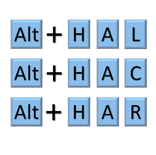
"Alt+H" will activate the "Home" tab in the ribbon and shortcut letters of this tab will get activated.

Thus, the letters mentioned below along with "Alt+H" will be shortcut keys for respective text alignment:

Vertical Alignment shortcuts:
AT-Align Top

AM-Align Middle

AB-Align Bottom

Also read: How to Trace Precedents and Dependents in Excel
Horizontal Alignment shortcuts:
AL-Align Left

AC-Align Center

AR-Align Right

Also read: How to Freeze Panes in Excel 2013

Once the alignment options are applied, the active alignment of the active cell can be seen in the alignment area as below:

More interesting articles on this website:

• Two-way Lookup in Excel 2013 using MATCH and INDEX
• How to create Histogram in Excel 2013
• How to insert current date and time in a cell in Excel 2013

How to use SUMPRODUCT function in Excel 2013

SUMPRODUCT is perfect formula if we have two or more arrays (range of cells in column/row) and you want to find the total value of the columns multiplied together.

Syntax:      =SUMPRODUCT(array1, [array2], [array3],...,[array255])

• array1: Data in the first column/row
• array2: Data in the second column/row and so on.

SUMPRODUCT formula can accommodate up to 255 arrays.

IMPORTANT NOTES:

• All the arrays should have same number of data entries. You can't have array1 containing 13 cells in a column, and array2 having only 12 cells. This will return #VALUE! error.
• Cells containing text OR blank cells are treated as zeroes by SUMPRODUCT function.

How to use SUBSTITUTE function in Excel 2013

SUBSTITUTE is very useful function in Excel when we want to replace specific text in a text string with some other text.

Syntax:               =SUBSTITUTE(text, old_text, new_text, [instance_num])

• text: The original text string containing the text to be replaced
• old_text: The text/data you want to replace with new_text
• new_text: The text/data that is used to replace the old_text
• [instance_num]: An option which specifies which occurance of old_text you want to replace

• If [instance_num] is specified, just that instance of the old_text is replaced;
• Otherwise, all instances of old_text are replaced with new_text.

IMPORTANT NOTES:

• The SUBSTITUTE function is Case Sensitive.
• The function can take texts, numbers as well as cell references for replacement.
• Text strings should always be placed using double quotes (eg. “Tom") while the reference cell formula (eg. C4) do not need double quotes. For numbers, using double quotes is optional.
• The output generated will always in text format, even if the input data were in number format.

How to generate RANDOM number in Excel 2013

Excel provides excellent functions to generate random numbers. RANDBETWEEN and RAND are two primary functions used to generate random numbers.

Using RANDBETWEEN Function:

This function returns random whole number between the given range.

Syntax:        =RANDBETWEEN(lower end of range, higher end of range)  OR
                    =RANDBETWEEN(bottom, top)

For example, to obtain a random number between 25 and 150 we enter as below:

=RANDBETWEEN(25, 150)

Using RAND Function:

This function returns a random decimal number between 0 and 1. Hence, (0,1) is the default range for the function.

Syntax:          =RAND()

To generate a random real number between a and b, you can use following formula:

=RAND()*(b-a)+a

For example, to generate real number between 25 and 150, use the formula below:

=RAND()*125+25     {the first part will give number between 0 to 125 which will then get added to 25}

IMPORTANT NOTES:

• The number generated by these functions will change each time we refresh the sheet or on pressing F9 button. To use these functions effectively, it should be combined with other functions like CHOOSE.
• If you want to use these functions to generate a random number but don't want the numbers to change every time the cell is calculated, you can enter =RAND()  or =RANDBETWEEN(a,b) in the formula bar, and then press F9 to change the formula to a permanent random number.