How to create a Scenario Summary Report in Excel 2013

After using Scenario Manager to add scenarios to a table in a worksheet, we can generate a summary report to visualize all the scenarios as well as scenario with current input values. The summary report show input values in different scenarios as well as the output generated (based on the selection).

1. Open the workbook containing the required scenarios.

2. Open the Scenario Manager dialog box.

Go To: “DATA” tab in the ribbon>> What-If Analysis>>>Scenario Manager [Shortcut: Alt+AWS]

3. Click on the "Summary" button in this dialog box.

A new dialog box will open giving the options to generate the summary report. The dialog box gives us choice of reports that can be generated: Scenario summary (static) and Scenario PivotTable report (dynamic).

After selecting the type of report, click on "Result cells" and select the result cell (required output).

4. Click "OK" to generate the report.

Excel creates a separate worksheet with input values along with selected result cells for all the scenarios as well as current input values. We can appropriately rename and re-position this Scenario summary worksheet and then save the workbook.

How to use Scenario Manager in Excel 2013

Scenarios form an important part in real-world problems. The inputs used in the real-world problems are dynamic and hence lead to different outputs. Scenario Manager in Excel help us in getting solutions of these problems by accounting for changing inputs. Before we create a scenario, we must design the worksheet so that it contains at least one formula that is dependent on the input cells.

Once various scenarios are created based on different input values, Excel provides facility to create a detailed summary report of these scenarios.

Let's understand this on the basis of Costing example. The example calculates Net revenue of a coffee shop.

Formula: Net revenue = Gross Revenue - Total Variable Cost - Total Fixed Cost

Where, Gross Revenue = (Number of coffee cups sold *Selling Price per unit);                                 Total Variable Cost = (Number of coffee cups sold*Variable cost per unit)

Let's name these input cells as Number_Units_Sold, Selling_Price_Unit, Variable_Unit, Total_Fixed

Go To: "DATA" tab in the ribbon>> What-If Analysis>>>Scenario Manager [Shortcut: Alt+AWS]

CREATING SCENARIOS:

1. Click on the "Add" button in the Scenario Manager dialog box.

Insert Scenario name as "Base Case" and select all the input values (C2:C5) in Changing Cells field. In case the input values are scattered, we can hold CTRL key while clicking on different input cells OR use comma after clicking on each input cell.

2. Click "OK". This will open Scenario Values dialog box.

Insert various input values corresponding to this scenario as shown above.

3. Click "Add" to insert new scenario OR click "OK" to stop adding scenarios.

Once all the scenarios are added, the Scenario Manager dialog box will open again and show names of all the entered scenarios.

4. To see result of a particular scenario, click on the Scenario name and press "Show" button.

Excel will automatically change input values as listed in the scenario and show relevant output.

IMPORTANT NOTE:

• Always assign range names to your input cells before you begin creating the various scenarios. It is easy to recognize the input filed by names while using the Scenario Values dialog box to enter input values for various scenarios.

How to use Goal Seek feature in Excel 2013

Goal Seek feature is an excellent tool in excel to obtain an input value for the desired output value for a given relationship between variables. This eliminates trial and error method to insert different set of input values to get desired output value and above all it's dynamic to use.

The word "Goal Seek" explains the feature that it will seek to find appropriate input value for desired goal (output).

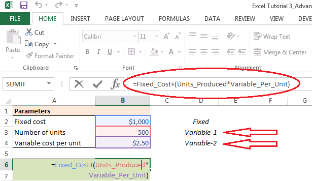
Let's straight away jump into an example of costing to understand it better. The example given here is used to calculate the Total Cost of the company for given variables i.e. Number of units produced and Variable cost per unit. For example, the fixed cost is $1,000 (cell B2), number of units is inserted in cell B3 (say 500) and variable cost per unit in cell B4 (say $2.5 per unit)

Output calculated as: [Fixed_Cost]+[Units_Produced*Variable_Per_Unit] OR = B2+(B3*B4)

The final output derived for this is in cell B6 (Total cost = $2,250).

Now, suppose I have certain budget for Total Cost (say $1800, the desired output) and I have to determine the Number of units that can be produced with this constraint (for given fixed cost and variable cost per unit assumptions).

Following steps will be useful to use Goal Seek the appropriate input value (Number of units) for desired Total Cost (output):

1. Select the cell whose value you wish to change.

This should be the cell that already contains a formula (here cell B6 which calculates Total Cost)

2. Go to Ribbon. Click...Data--->What-if Analysis--->Goal Seek [ Shortcut: Alt+AWG ]

This will show a Goal Seek dialog box on the Excel screen.

4. The dialog box will have three fields as below:

Set Cell: The cell that will contain the desired output (cell B6 with formula that is already selected)

To Value: Insert the desired output that is required (here 1800, the
value of Total Cost)

By Changing Cell: The cell with input value that needs to be changed as per desired output (Units)

5. Click Ok.

On clicking "OK", a new dialog box showing the status of the analysis will be populated.

IMPORTANT NOTE:

• The status dialog box informs that goal seeking process a found the solution. When this is not the case, the Step and Pause buttons inside the dialog box become visible, and further iterations could be carried to narrow and ultimately get the desired value.

Click "OK" to keep the values. Click "Cancel" in case you want to return to original values

How to create a Two-Variable Data Table in Excel 2013

Two-variable data table is an excellent tool in excel to perform sensitivity analysis with two ranges of possible input values. It helps in getting output for dual range of input values for given formula. This avoids repeating the formula for each of the range of input values and above all it's dynamic to use.

The formulas in a two-variable data table refer to two input cells and shows corresponding output. We can insert a range of values for the Row Input Cell across the first row of the table and range of values for the Column Input Cell down the first column of the table.

Also read: How to create One-Variable data table in Excel 2013

Let's straight away jump into an example of costing to understand it better. The example given here is used to calculate the Total Cost of the company for two variables i.e. Number of units produced and Variable cost per unit (assuming fixed cost as constant).

For example, the fixed cost is $1,000 (cell B2), number of units is inserted in cell B3 (say 500) and variable cost per unit in cell B4 (say $2.5 per unit)

Output calculated as: [Fixed_Cost]+[Units_Produced*Variable_Per_Unit] OR = B2+(B3*B4)
The final output derived for this is in cell B6 ($2,250).

Now, the two-variable data table is useful when you want resultant Total Cost for different number of units produced and different variable cost per unit (sensitivity analysis). Let's insert the range of units ranging 100 to 1,000 in column C in the cell range C10:C19 and similarly range of Variable cost per unit 1.0 to 5.0 in Row 9 in the cell range D9:L9.

Following steps will be useful to create two-variable data table that will give Total Cost for different inputs of Units produced and Variable cost per unit:

1. Copy the formula for calculation (originally in cell B6) into cell C9 (at the intersection of row and column of inputs) by typing =(equal to) and then clicking cell B6 (to create formula reference for your output)

This enables the table function to understand what formula to apply on the input cell in order to get the output.

2. Select data range C9:L19.

This range includes input variables, the formula linked in step-1 and range desired for output variables.

3. Go to Ribbon. Click...Data--->What-if Analysis--->Data Table  [ Shortcut: Alt+AWT ]

This will show a Data Table dialog box on the Excel screen.

4. Click on the Row Input Cell text box in the dialog box and then select cell B4 by clicking it (since the input values of "units" is inserted in row). Similarly, click on Column Input Cell text box and select B3
This will insert absolute cell reference $B$4 of the formula into Row Input Cell text box and  $B$3 of the formula into the Column Input Cell text box of the dialog box.

5. Click Ok.
On clicking "OK", the dialog box will get closed. On minute look into the formula bar, the cell range C9:L19 will show TABLE function.

6. Copy format to the output range by Format Painter.
Alternatively, copy from original output (cell B6) and paste format into output range
[Shortcut: Alt+EST]

IMPORTANT NOTES:

• The output cell range (here C9:L19) will show TABLE function with formula cell (B4,B3) inside {} brackets. This means it is an array. Hence, you cannot delete part of this range (will throw error while doing so). To delete or clear the content it is necessary to select entire range.

• The input ranges are dynamic. If you change the input variables, it will automatically change the output variable.

• If the excel is in automatic mode, all the data table gets updated each time you refresh or save the excel workbook (and this may be irritating sometimes..!!). In order to prevent Excel from updating these data table until we Refresh (F9) or Calculate sheet (Shift+F9) on the Formulas tab,

Go to File--->Options--->Formulas--->Workbook Calculation--->Automatic except for Data Tables
[Shortcut: Alt+MXE]

OR Go to "FORMULAS" tab >>> Calculation Options >>> Automatic except for Data Tables

More interesting articles on this website:

• Text Alignment keyboard shortcuts for Excel 2013
• How to freeze panes in Excel 2013
• How to generate RANDOM number in Excel 2013

How to create a One-Variable Data Table in Excel 2013

One-variable data table is an excellent tool in excel to perform what-if analysis. It helps in getting output for series of input values for given formula. This avoids repeating the formula for each of the input value and above all it's dynamic to use.

The formulas in a one-variable data table refer to only one input cell and shows corresponding output. We can insert different input variables either in a row or a column. The ouput will be available in the next row or column as the case may be.

Also read: How to create a Two-Variable Data Table in Excel 2013

Let's straight away jump into an example to understand it better. The example given here is used to calculate the YoY population growth of country X. For example, the population in 2012 is 5,955 million (cell B2), the growth rate is inserted in cell B3 (say 3.25%).

Output calculated as: [Population_2012]+[Growth_Rate*Population_2012]    OR  = B2+(B3*B2)

The final output derived for this is in cell B5 (6,149 million in 2013).

Now, the one-variable data table is useful when you want resultant population in 2013 for different growth rates (what-if analysis). Let's insert the range of growth rates ranging 1% to 10% in column C in the cell range C10:C19 (same could be done for a row).

Following steps will be useful to create one-variable data table that will give population in 2013 for different inputs of growth rates:

1. Copy the formula for calculation (originally in cell B5) into cell C9 (on the top of output column) by typing =(equal to) and then clicking cell B5 (to create formula reference for your output)

This enables the table function to understand what formula to apply on the input cell in order to get the output.

2. Select data range B9:C19.

This range includes input variables, the formula linked in step-1 and range desired for output variables.

3. Go to Ribbon. Click...Data--->What-if Analysis--->Data Table [ Shortcut: Alt+AWT ]

This will show a Data Table dialog box on the Excel screen.

4. Click on the Column Input Cell text box in the dialog box (Row Input Cell text box in case output is needed in row) and then select cell B3 by clicking it (the cell with original formula)

This will insert absolute cell reference $B$3 of the formula into the Column Iput Cell text box of the dialog box

5. Click Ok.

On clicking "OK", the dialog box will get closed. On minute look into the formula bar, the cell range C9:C19 will show TABLE function.

6. Copy format to the ouput range by Format Painter

Alternatively, copy from original output (cell B5) and paste format into output range[Shortcut: Alt+EST]

IMPORTANT NOTES:

• The output cell range (here C9:C19) will show TABLE function with formula cell (B3) inside {} brackets. This means it is an array. Hence, you cannot delete part of this range (will throw error while doing so). To delete or clear the content it is necessary to select entire range.

• The input range is dynamic. If you change the input variables (B9:B19), it will automatically change the output variable.

• If the excel is in automatic mode, all the data table gets updated each time you refresh or save the excel workbook (and this may be irritating sometimes..!!). In order to prevent Excel from updating these data table until we Refresh (F9) or Calculate sheet (Shift+F9) on the Formulas tab,

Go to File--->Options--->Formulas--->Workbook Calculation--->Automatic except for Data Tables
[Shortcut: Alt+MXE]

OR        Go to Formulas tab--->Calculation Options--->Automatic except for Data Tables

More interesting articles on this website:

• How to use Scenario Manager in Excel 2013
• How to freeze panes in Excel 2013
• How to generate RANDOM number in Excel 2013
• How to use AGGREGATE function in Excel 2013